Data Science : Faster approximate neighbourhood search with Locality Sensitive Hashing

Reducing time complexity of KNN by using an approximation algorithm

# ref — https://erikbern.com/2015/09/24/nearest-neighbor-methods-vector-models-part-1.html

1) The Problem with KNN

If you have to perform a neighbourhood search, you would have to go through all the points in your dataset and calculate distances between each and get the first K nearest neighbours with least distances. This would cost a run time complexity of O(n*d) since you would run through each of the ’n’ training data points and each point being a ‘d’ dimensional entity. So if you have a large data to scan, this would take forever to run. A better solution to this is to use Locality Sensitive Hashing which is an approximation algorithm. Let’s take an example where you have the following set of points in a 2D space. To keep things simple, we will take 2-dimensions for now.

point set in 2D space

2) Locality Sensitive Hashing (LSH)

What this does is it partitions the space into multiple regions by using seperating hyperplanes. Think of it as you are trying to slice a large pizza into sub regions by slicing each cut of the pizza across the diameter.

subspaces obtained by random hyperplane partitioning

Here, we can see above that we have used 8 random hyperplanes (Let ‘M’ be the number of hyperplanes used) to partition our space into (2*M) subspaces/regions/slices in the 2D space. So, in this case we have 2*8 = 16 subspaces.

For generating random hyperplanes, you can use the equation of a hyperplane as (wTx + b = 0) where each of the w are sampled from a Gaussian random N(0,1) to obtain the stochasticity in the hyperplanes that are generated.

Now, you can think of each slice as a local neighbourhood in space. If you were in a 2D world, this assumption would hold true intuitively as it is easier to imagine as well. Now, how do we represent each of these 16 subspaces ?

We can go back to our high school linear algebra and get the answer. If you think about it intuitively, each of the 16 subspaces that we have obtained can be represented as a 8 dimension vector (number of hyperplanes) because each of these subspace either lies on the positive or negative side of each of the hyperplanes. So ,we just take the sign of (wTx + b) — if this is > 0, it indicates it lies on the right side and if it is < 0, it indicates that it lies on the left side of the hyperplane. Let’s have a sign function which returns +1 if it lies on the right side and return -1 if it lies on the negative side.

# ref — https://medium.com/analytics-vidhya/fundamentals-of-logistic-regression-bde451712652

So basically, we can represent each of our subspaces as follows —

LSH — subspaces representations

So, we can see that Region 1 (R1) in the figure above is represented as [-1,+1,-1] since all the points in Region R1 — if you apply the function sign(wTx + b) across each of the hyperplane, you get this result.

The way you construct the above m-dimensional vector for each of the subspaces is —

for hyperplane 1 = sign(w1Tx + b)

for hyperplane 2 = sign(w2Tx + b)

…….

for hyperplane 8 = sign(w8Tx + b)

and then construct the 8 dimension vector as above. Ideally, you can neglect the intercept term since I have taken a simple case where all the hyperplanes passing through origin so you can take b = 0.

So you have obtained the 16 hash buckets ([-1, +1, +1]) for each subspace. Now, we can just store this in a key-value store where your key would be the hash-bucket that you have obtained and values could be the point indices of all the training data points in your training dataset.

3) Accounting for Approximation & Stochasticity in the LSH output

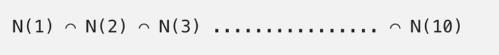
Now, you must have understood that LSH gives multiple outputs each time you run because you are generating random hyperplanes which are being sampled from a normal distribution. So, every time you run LSH with same hyper-parameters, you get different outputs. To tackle this stochasticity, we run the LSH algorithm multiple times in our dataset and then for a query point, we choose the intersection set of points across all LSH algorithms as our neighbours because we want to be sure that a given point is a neighbour if and only if the point stays consistent with random hyperplane slicings.

For a given query point xq during run time,

N(xq, LSH 1) — {x1, x3, x6, x8, x9}

N(xq, LSH 2) — {x5, x3, x8, x15}

…..

N(xq, LSH 10) — {x1, x3, x8, x17, x19}

So our final neighbourhood set can be treated as N(xq) = {x3, x8} as these are the only 2 points that stay consistent across all the 10 LSH generators. You can also choose to have more neighbours but need to limit the number of LSHs you run because the more times you run, your neighbourhood set would narrow down but your confidence about the neighbourhood set being actually a neighbourhood of the query point will increase.

4) Results obtained with LSH on the dataset

As you can see if we run LSH on the above dataset for a query point, we are able to find the nearest neighbours. The green point represents the query point whereas the blue points represent the neighbours. Please note here that neighbours here are calculated with respect to Cosine similarity and not Euclidean distance. So basically, the neighbours that are obtained here are basis angular similarity of vectors and not the euclidean L2 distance.